What is RK4?

Runge-Kutta methods are a family of iterative methods, used to approximate solutions of Ordinary Differential Equations (ODEs).

Such methods use discretization to calculate the solutions in small steps. The approximation of the “next step” is calculated from the previous one, by adding s terms.

An actual, in-depth analysis could be the subject of a whole book, but in this post, I’d like to show a graphical overview of how the most popular member of this family works.

Let’s get to it!

The fourth-order Runge-Kutta method also known as “RK4” or “the Runge-Kutta method” is one of the most (if not the most) popular method of solving ODEs. It provides a very good balance between computational cost and accuracy. It is used as a solver in many frameworks and libraries, including SciPy, JuliaDiffEq, Matlab, Octave and Mathematica.

Beyond fourth-order methods, the gain in accuracy is offset by the complexity. For RK1 through RK4, the number of steps (or stages) required is the same as the order, but that doesn’t hold for higher-order versions (eg. RK4 : 4 steps, RK5 : 6 steps).

As we mentioned Runge-Kutta is a collection of methods. The n-order case requires s free parameters, one for each stage for an implementation, also known as the Butcher tableau.

RK1, with one stage, is equal to Euler’s method.
RK2, with two stages, can be implemented as Heun’s Method, the Midpoint Method, or Ralston’s Method, depending on the tableau.

The figure is adapted from Prof. Kosmidis’ lectures for the Numerical Analysis course at my MSc program.

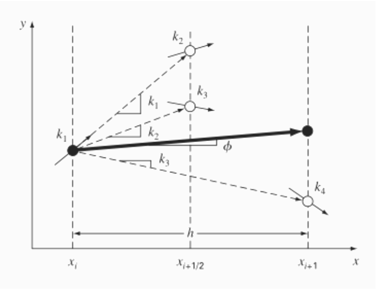
We start from point y=f(xi) and wish to approximate f(xi+h)

Step 1:
Start from y, with the initial k1 approximation from Euler’s method, evaluate at the midpoint, finding k2.
Step 2:
Start from y with k2, and re-evaluate at the midpoint, finding k3.
Step 3:
Start from y with k3, and evaluate at the endpoint, finding k4.
Step 4:
The approximation of the “next step” is given by weighted average of these four k-values as

The local truncation error is O(h^5), while the total accumulated error order is O(h^4).

What’s more?

A lot more could be said about the order of the errors versus order of the methods, adaptive and implicit Runge-Kutta variants, stability of various implementations. I hope to find the time to write about cool stuff like this soon!